An Incremental Scheme for Dictionary-based Compressive SLAM

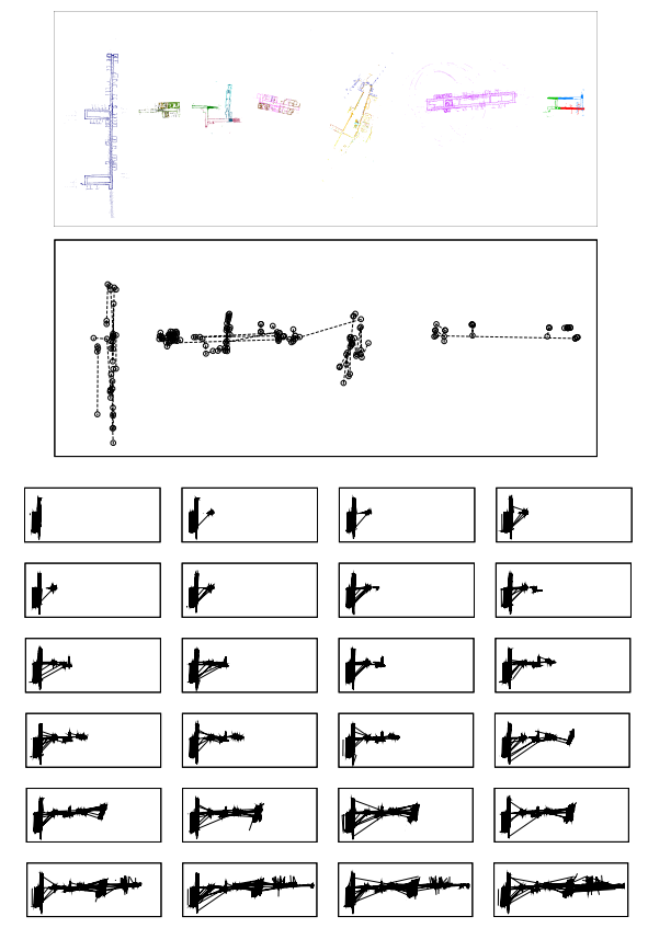
Fig. 1. Incremental map compression. The input is a sequence of submaps built by mapper robots during a SLAM task (top figure, 24 submaps, each is distinguished by different colors). A set of datapoints are compactly represented in the form of compression trajectory, a sequence of transformed datapoints (middle figure, random 100 examples of compression trajectories). The incremental map compression is a process of updating a set of compression trajectories by incorporating latest submap (bottom figures, respectively corresponding to the 1st, 2nd, ..., 24th update).

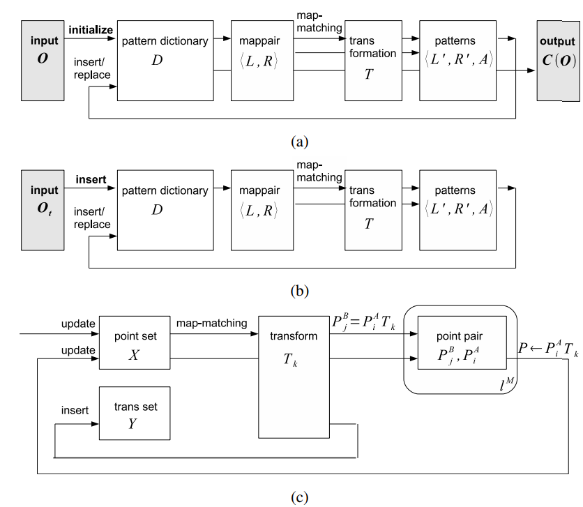
Fig. 2. Overview. (a) Batch map compression task addressed in [1] [2]. Patterns in the dictionary are recursively explained by smaller patterns. It was assumed that compression of pattern dictionary is performed after finding repetitive patterns has been finished. (b) Incremental map compression task addressed in the current paper. It is required that compression has to be performed while simultaneously finding repetitive patterns. (c) The incremental map compressor.

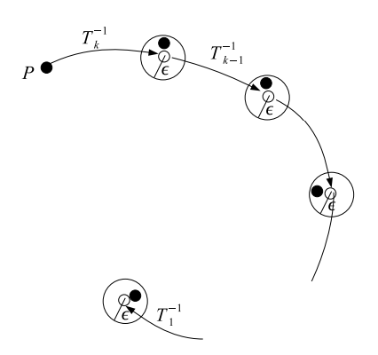
Fig. 3. Compression trajectory. A compression trajectory represents a sequence of transformed datapoints. Each point on the trajectory is an approximation of an original datapoint. The approximation error is smaller than ε and free from error accumulation.

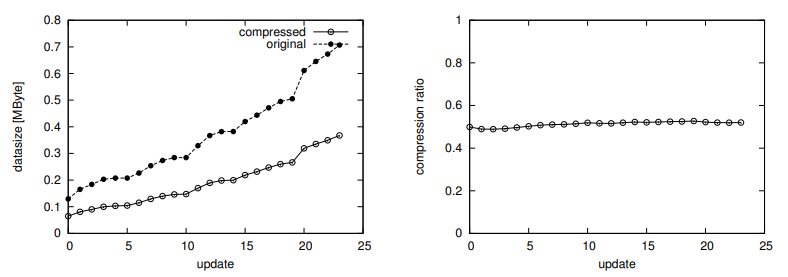
Fig. 4. An example of compression result. Left: datasize of compressed and original data. Right: compression ratio.

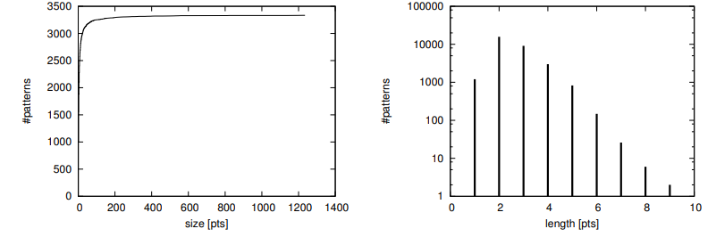
Fig. 5. Statistics of repetitive patterns. Left: size of patterns, a cumulative histogram of number of datapoints in each pattern. Right: length of compression trajectories, a frequency histogram.

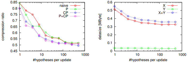
Fig. 6. Compression performance. Left: compression ratio of the final map (i.e. after 24th update) vs. resource (#hypotheses) per update, for four different map matching strategies “naive”, “P”, “CP” and “P+CP”. Right: datasize [MByte] of X and Y (for the strategy “P+CP”).

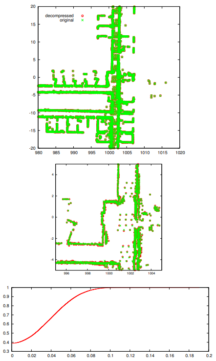
Fig. 7. A decompression result. Top: the decompressed map superimposed on the original map. Bottom: accumulative frequency of spatial error [m].

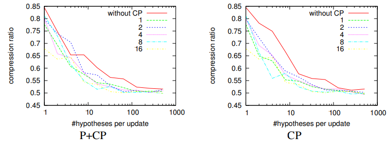
Fig. 8. Results for various feature size χ[m] for the CP visual search.

Fig. 9. Comparison between map-matching strategies, “naive”, “P”, “CP” and “P+CP”. The vertical axis: average computation time [sec] per update (i.e. per 100 map-matching). The horizontal axis: timestamp t (update ID).

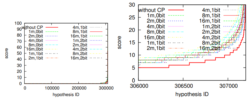
Fig. 10. Comparison between a strategy with CP (“P+CP”) and a strategy without CP (“P”). The strategy “P+CP” is investigated for several different settings of the parameters χ and α (0bit, 1bit or 2bit). For clarity, hypotheses are aligned in the ascending order of their scores. The right figure is a closeup of the left figure.

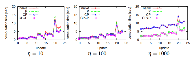
Fig. 11. Map compression cost [sec]. The vertical axis: average computation time [sec] per update (100 map-matching). The horizontal axis: timestamp t (update ID).

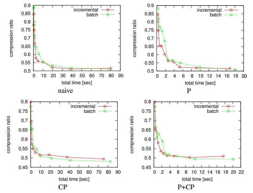
Fig. 12. Incremental vs. batch. Either scheme is investigated for several different settings of number of hypotheses η. The horizontal axis: computation time [sec] spent. The vertical axis: compression ratio of the final map (i.e. after 24th update).

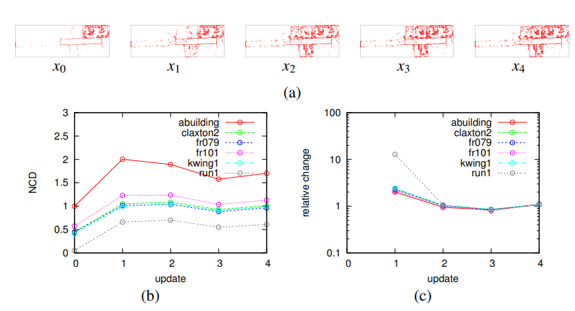
Fig. 13. Incremental estimation of NCD. NCD between mappairs is incrementally estimated while simultaneously building the map. The map xt (t = 0,1,2,3,4) is incrementally built by incorporating the five submaps from “albert”, as shown in Fig.a. The estimate NCD(xt ,y) of NCD between latest map xt and each database map y (“abuilding”, “claxton2”, “fr079”, “fr101”, “kwing1”, “run1”) is incrementally updated at each time t, as shown in Fig.b. Fig.c visualizes relative change in NCD: NCD(xt , y)/NCD(xt−1, y). One can see that the NCD score converges even at the early stages of the map building task, e.g. t = 1,2.