Dark Reciprocal-Rank: Teacher-to-student Knowledge Transfer from Self-localization Model to Graph-convolutional Neural Network
Takeda Koji Tanaka Kanji
Keywords
Abstract
In visual robot self-localization, graph-based scene representation and matching have recently attracted re- search interest as robust and discriminative methods for self- localization. Although effective, their computational and storage costs do not scale well to large-size environments. To alleviate this problem, we formulate self-localization as a graph classi- fication problem and attempt to use the graph convolutional neural network (GCN) as a graph classification engine. A straightforward approach is to use visual feature descriptors that are employed by state-of-the-art self-localization systems, directly as graph node features. However, their superior performance in the original self-localization system may not necessarily be replicated in GCN-based self-localization. To address this issue, we introduce a novel teacher-to-student knowledge-transfer scheme based on rank matching, in which the reciprocal-rank vector output by an off-the-shelf state-of- the-art teacher self-localization model is used as the dark knowl- edge to transfer. Experiments indicate that the proposed graph- convolutional self-localization network (GCLN) can signifi- cantly outperform state-of-the-art self-localization systems, as well as the teacher classifier. The code and dataset are available at https://github.com/KojiTakeda00/Reciprocal rank KT GCN.
Related document
BibTeX
@inproceedings{DBLP:conf/icra/TakedaT21,
author = {Koji Takeda and
Kanji Tanaka},
title = {Dark Reciprocal-Rank: Teacher-to-student Knowledge Transfer from Self-localization
Model to Graph-convolutional Neural Network},
booktitle = {{IEEE} International Conference on Robotics and Automation, {ICRA}
2021, Xi'an, China, May 30 - June 5, 2021},
pages = {1846--1853},
publisher = {{IEEE}},
year = {2021},
url = {https://doi.org/10.1109/ICRA48506.2021.9561158},
doi = {10.1109/ICRA48506.2021.9561158},
timestamp = {Thu, 14 Sep 2023 17:57:15 +0200},
biburl = {https://dblp.org/rec/conf/icra/TakedaT21.bib},
bibsource = {dblp computer science bibliography, https://dblp.org}
}
図表・写真
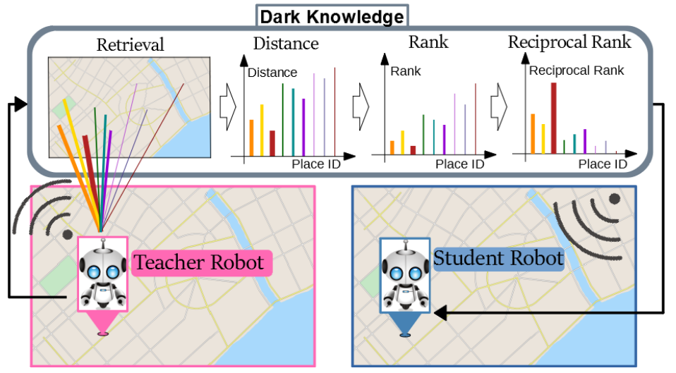
Fig. 1. We propose the use of the reciprocal-rank vector as the dark knowledge to be transferred from a self-localization model
(i.e., teacher) to a graph convolutional self-localization network (i.e., student), for improving the self-localization performance.
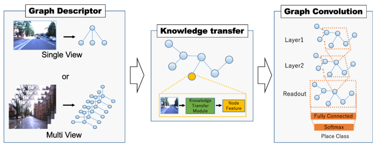
Fig. 2. System architecture.
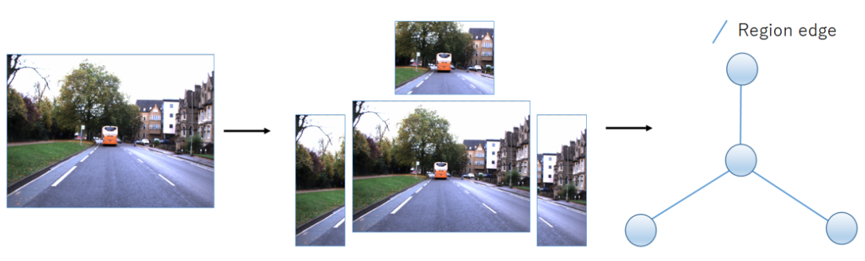
Fig. 3. Single-view subimage-level scene graph (SVSL).
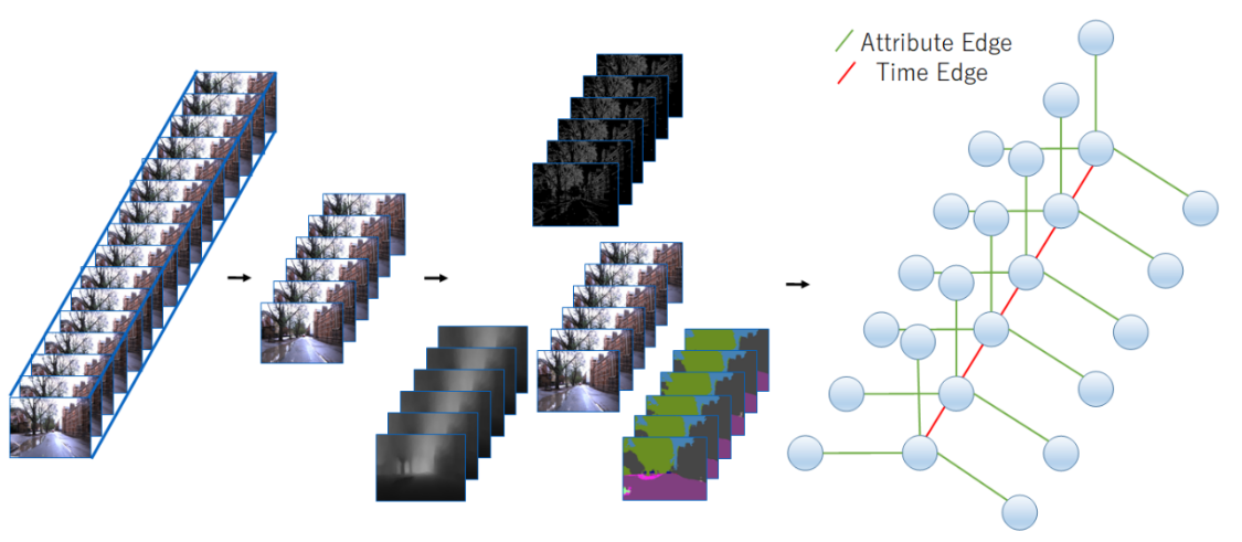
Fig. 4. Multi-view image-level scene graph (MVIL).
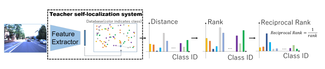
Fig. 5. Knowledge transfer on node feature descriptor.
Table1:STATISTICS OF THE DATASET.
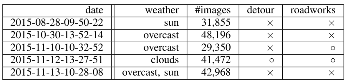
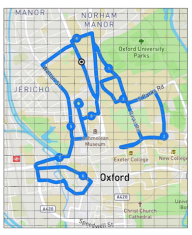
Fig. 6. Example of place partitioning.
Table2:AVERAGE TOP-1 ACCURACY.
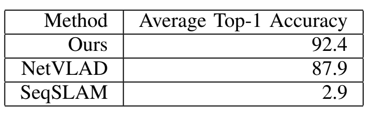
Table3:PERFORMANCE RESULTS VERSUS THE GRAPH STRUCTURE.
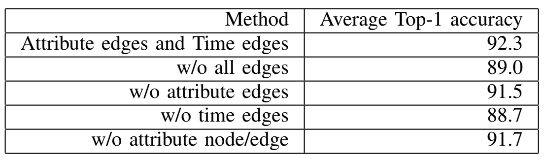
Table4:PERFORMANCE RESULTS FOR DIFFERENT COMBINATIONS OF K AND IMAGE FILTERS.
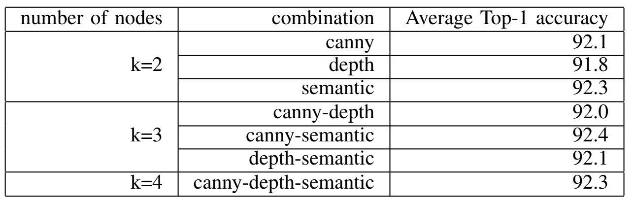
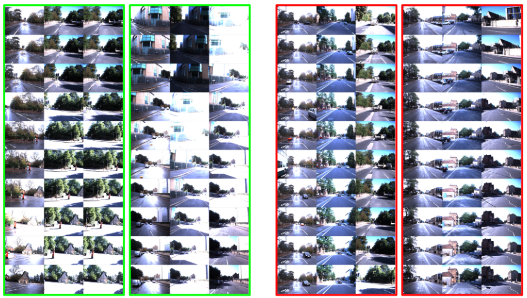
Fig. 7. Example results. From left to right, the panels show the query scene, the top-ranked DB scene,
and the ground-truth DB scene. Green and red bounding boxes indicate “success” and “failure” examples, respectively.
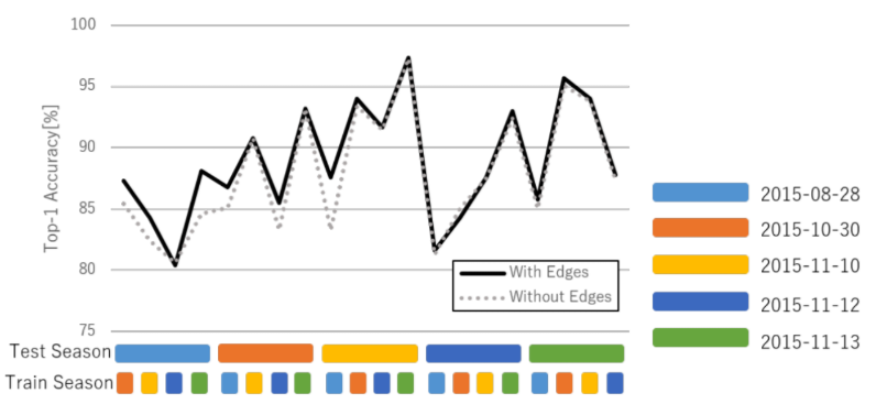
Fig. 8. Performance results for single-view scene graph with and without edge connections.
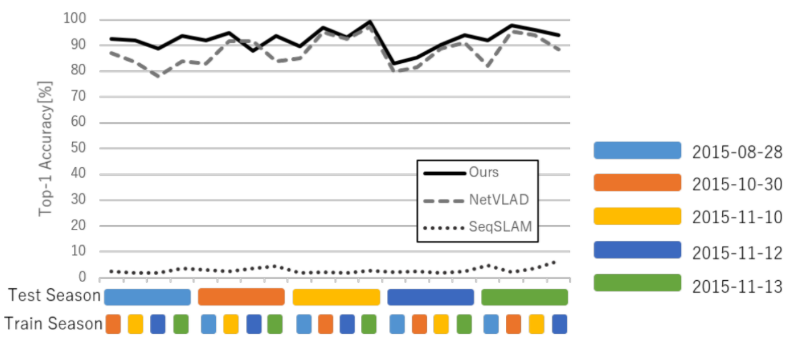
Fig. 9. Performance results for different training and test season pairs.
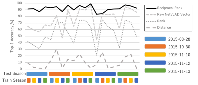
Fig. 10. Performance results versus the choice of attribute image descriptors (K=2).
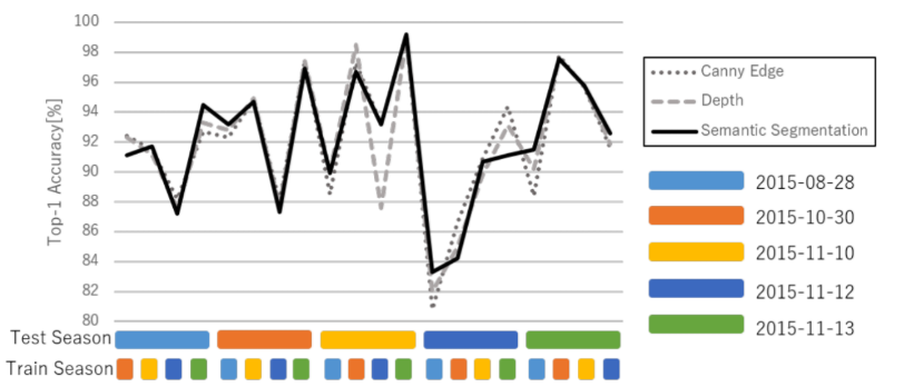
Fig. 11. Performance results for individual training/test season pairs (K=2).