Visual Robot Localization Using Compact Binary Landmarks
Kouichirou Ikeda, Kanji Tanaka
Keywords
Abstract
This paper is concerned with the problem of mobile robot localization using a novel compact representation of visual landmarks. With recent progress in lifelong maplearning as well as in information sharing networks, compact representation of a large-size landmark database has become crucial. In this paper, we propose a compact binary code (e.g. 32bit code) landmark representation by employing the semantic hashing technique from web-scale image retrieval. We show how well such a binary representation achieves compactness of a landmark database while maintaining efficiency of the localization system. In our contribution, we investigate the costperformance, the semantic gap, the saliency evaluation using the presented techniques as well as challenge to further reduce the resources (#bits) per landmark. Experiments using a high-speed car-like robot show promising results.
Related document
BibTeX
@inproceedings{DBLP:conf/icra/IkedaT10,
author = {Kouichirou Ikeda and
Kanji Tanaka},
title = {Visual robot localization using compact binary landmarks},
booktitle = {{IEEE} International Conference on Robotics and Automation, {ICRA}
2010, Anchorage, Alaska, USA, 3-7 May 2010},
pages = {4397--4403},
publisher = {{IEEE}},
year = {2010},
url = {https://doi.org/10.1109/ROBOT.2010.5509579},
doi = {10.1109/ROBOT.2010.5509579},
timestamp = {Tue, 20 Feb 2024 13:40:10 +0100},
biburl = {https://dblp.org/rec/conf/icra/IkedaT10.bib},
bibsource = {dblp computer science bibliography, https://dblp.org}
}
図表・写真
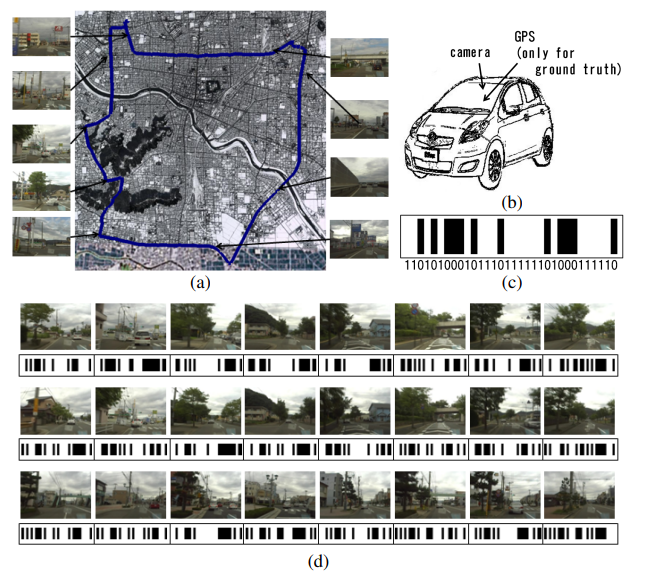
Fig. 1. How well compact binary landmark representation works in mobile robot localization? (a) Experimental environment and robot’s trajectory.
(b) A high-speed car-like mobile robot. (c) Binary landmark representation using the semantic hashing technique. (d) Sequences of images and binary codes.
Top, Middle: Two similar locations. Bottom: A dissimilar location. Note that the codes are similar/dissimilar only at a few bits.
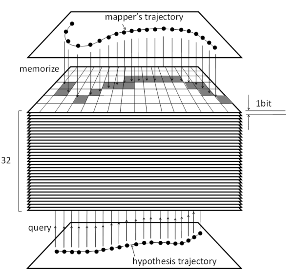
Fig. 2. Binary maps. Individual binary codes are viewed as different type independent measurements. We employ K different binary maps
for K bit code and then record i-th bit measurements on i-th map. We also discuss how many K ′ (< K) binary maps are required for successful localization.
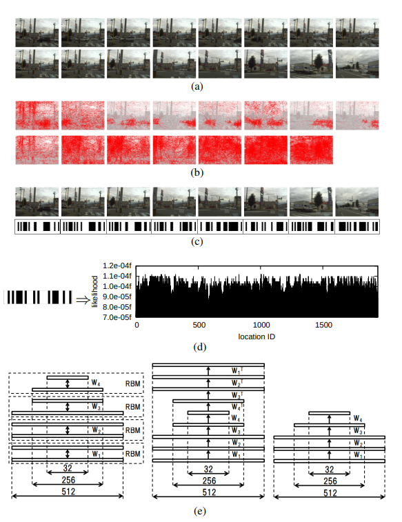
Fig. 3. Visual localization processing. (a) Input images. (b) Optical flows. (c) Binary codes. (d) Observation likelihood over the robot pose space.
(e) Semantic hashing architecture. Left: Pre-training. Middle: Fine-tuning. Right: Encoding. The number of nodes for each layer is also shown in the figures.
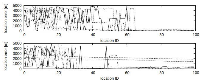
Fig. 4. Localization errors for 5 success examples (top) and for 5 failure examples (bottom), randomly sampled from the 100 localization tasks.
Vertical axis: location error [m]. Horizontal axis: location ID.
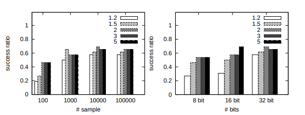
Fig. 5. Success ratio vs. #samples (left) and success ratio vs. #bits (right) over the 100 tasks. Each plot corresponds to each value of parameter cL.
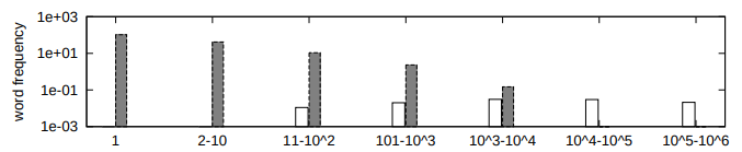
Fig. 6. Word frequency of ”Outdoor” dataset (left) vs. ”LabelMe” (right).
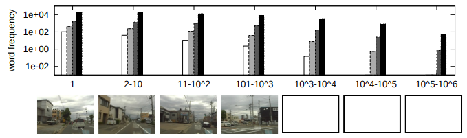
Fig. 7. Frequency of visual words. Top: Average number of landmarks per word. Words are sorted in terms of the number of landmarks
they contain and then grouped into 7 groups. Each datapoint from left to right respectively corresponds to the word as well as their
near neighbors in terms of Hamming distance 1, 2 and 3. Bottom: Images corresponding to the central words (ID: 1, 5, 50 and 500) of each group.
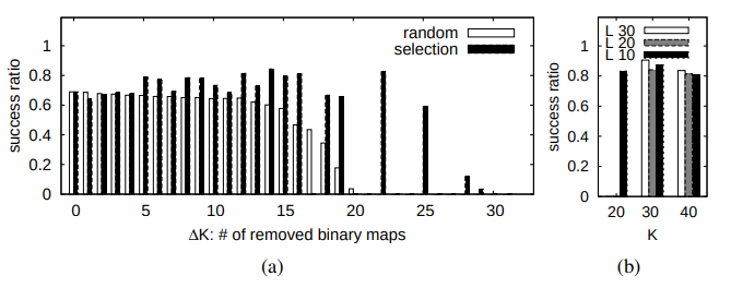
Fig. 8. Localization performance. (a) The semantic hashing localization. Left: The random sampling strategy. Right: The planned sampling strategy.
Vertical axis: success ratio. Horizontal axis: the number ∆K of removed binary maps. (b) The LSH-based localization [9]. In some settings
(e.g. {∆K:22,”random”}, {L:20,K:20}), the success ratio is unreliable (due to low convergence rate) and omitted.